|    .  ___  __   __   ___ .  __      __   __        __   __   __
|    | |__  |__) |__) |__  ' /__`    /__` /  \  /\  |__) |__) /  \ \_/
|___ | |___ |  \ |  \ |___   .__/    .__/ \__/ /~~\ |    |__) \__/ / \
⋅∽⋅∼⋅∽⋅∼⋅∽⋅∼⋅∽⋅∼⋅∽⋅∼⋅∽⋅∼⋅∽⋅∼⋅∽⋅∼⋅∽⋅∼⋅∽⋅∼⋅∽⋅∼⋅∽⋅∼⋅∽⋅∼⋅∽⋅∼⋅∽⋅∽⋅∼⋅∽⋅∽⋅∽⋅∽⋅
We're creating a little program that takes in a soundfile, estimates the pitch and returns it as human readable notation. See previously:
specification and motivation
implementation planning
dev log 0
dev log 1
Last log was not very successful. Right now, the program we have has several big defaults with regards to our goals. Long story short, the basic data pipeline from sample to music notes works, but its performance is really bad. It also has a big defect: it only works if the notes are separated with silence. Which is a big constraints with regards as to what I want to use this program for. I want to sing the little tunes in my head as freely as possible, record them, pipe them in, get the notation out. If I have to focus on spacing each note, I tend to lose track of the little tunes.
Anyway, so let's change approaches by reframing the problem and start programming from scratch.
The spec that was defined is as follows:
- use a command line interface
- allow the user to feed a .wav as an external file
- analyse the pitch in that .wav
- print out the pitch as string ("c3 e3 g3" for instance)
- accidentals shall all be detected as sharps, not flats (like in the tracker I use)
The hard part is, of course, the pitch analysis. We use the pyin algorithm for that and we get the fundamental frequency of the sample as good as it gets. Let's call the array of the pyin detected frequencies over time the raw pitch, for the sake of simplicity.
On the other end of the pipeline, we have the music notation. What does it mean from a signal perspective? Music notation essentially assumes that the pitch will be held constant for periods of time corresponding to each note. From my understanding, each note is basically a boxcar function, with y the pitch and x the time. The information that we are trying to extract from the recorded sample is therefore a sum of boxcars. We can see this in the audioPulse pitch estimation example, especially in the ground truth encoding.
So the problem that we'll focus on is this transformation: how to we go from the pyin output to a sum of boxcars?
I have trust issues with the ground truth I generated before. But I trust in the sanctity of Twinkle, Twinkle Little Star. The melody is actually from a piece of Mozart himself, so we can't go wrong here. It starts:
c3 c3 g3 g3 a3 a3 g3 f3 f3 e3 e3 d3 d3 c3
Hence the detected music sheet should be c3 g3 a3 g3 f3 e3 d3 c3, as we don't focus on note duration yet.
This time, I encode it again on the M8 tracker, but this time, I control each note with a pitch detection app (side note, if I was patient, I guess I could achieve my goals directly with just a pitch detection app, but pausing for each notes breaks the flow). And indeed, the M8 is playing in tune and post recording through Audacity, it also appears to be ok.
So here we are, with our twinkle.wav and full of new resolve.
We'll go from the detected frequency and start processing it to shift it to the underlying reality we know it contains. In order to better see what we're doing, we'll use jupyter and our good old friend matplotlib
# in our virtual environment (cf dev log 1)
pip install jupyter # for interactive python notebooks
pip install matplotlib # for plots
	jupyter lab # start a little web server so we can use the browser interface
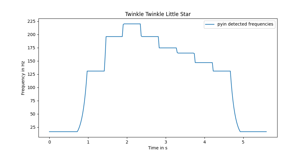
Let's load the sample, use pying and do a little plotting.
import librosa
import matplotlib.pyplot as plt

y, sr = librosa.load("twinkle.wav")

f0, voiced_flag, voiced_probs = librosa.pyin(y,
                                             sr=sr,
                                             fmin=librosa.note_to_hz('C0'),
                                             fmax=librosa.note_to_hz('C9'),
                                             fill_na=None)
times = librosa.times_like(f0)

f,a = plt.subplots()
a.plot(times,f0,label="pyin detected frequencies")
a.legend()
a.set_xlabel("Time in s")
a.set_ylabel("Frequency in Hz")
a.set_title("Twinkle Twinkle Little Star")

And... well I thought I would have to do more processing? The signal is already in great shape. I guess the ground truth is too simple this time? I guess I'll try doing a voice sample with the same tune to face the problem of less perfect instruments. But in the mean time, let's transform that signal into a partition we can use.
Right now, the signal is close to perfect. But perfect it is not. Note the ramps from one note to another, while the music sheet is pure box plots. Scipy has plenty of useful filters, and the doc recommends the image ones (they handle 1 dimensional inputs as well).
What I want would be some form of filter that looks at a signal bit and imposes the most representative entry as the right one.
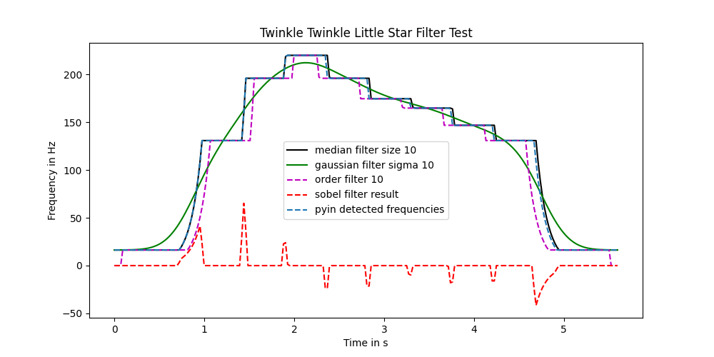
My signal processing classes are long gone, so I plotted them and had a look. First, I thought the median filter would be promising, but it's not doing what I need for the signal ramps. The Sobel filtering is interesting for a different purpose than what I seek right now (basically, it is meant for edge detection, which here means it can be used to separate notes time wise).
Then I thought that the order_filter is what I am looking for. I implemented it, tried different kernel sizes. But I am pretty unimpressed with the results. It does what the idea in my head said it should do, but this is far from good enough. Plus, in the case of the voice sample, the recorded frequency will oscillate around the intended one. Hence an order filter might not work great.
Here's an image of the attempt.
import numpy as np
import scipy.ndimage as sim
import scipy.signal as sig
filtered_f0 = sim.median_filter(f0,size=10)

f,a = plt.subplots()
a.plot(times,sim.median_filter(f0,size=10),label="median filter size 10", color= 'k')
a.plot(times,sim.gaussian_filter1d(f0,sigma=10),label="gaussian filter sigma 10", color='g')
a.plot(times,sig.order_filter(f0,domain=np.ones((1,11))[0],rank=1),color="m",linestyle="--",label="order filter 10")

a.plot(times,sim.sobel(f0),label="sobel filter result",color="r",linestyle="--")
a.plot(times,f0,label="pyin detected frequencies",linestyle="--")

a.legend()
a.set_xlabel("Time in s")
a.set_ylabel("Frequency in Hz")
a.set_title("Twinkle Twinkle Little Star Filter Test")
f.set_size_inches(10,5)
f.savefig("twinkle_twinkle_little_star_sample_filter_test.png")

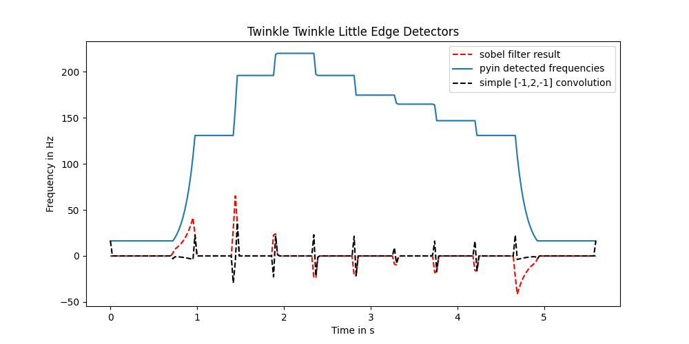
Given that I am missing something, I decided to open up some lectures on signal processing online, precisely on image processing given that what I am trying to do is similar to sharpening an image. I tried some kernels for sharpening and then I finally understood that I should be very humble in my estimation of my cognitive abilities. Namely, if I do a simple kernel such as [-1,2,-1], I have something very like the Sobel filter.
f,a = plt.subplots()
a.plot(times,sim.sobel(f0),label="sobel filter result",color="r",linestyle="--")
a.plot(times,f0,label="pyin detected frequencies",linestyle="-")
a.plot(times,sig.convolve(f0,[-1,2,-1],mode="same"),color="k",linestyle="--",label="simple [-1,2,-1] convolution")

a.legend()
a.set_xlabel("Time in s")
a.set_ylabel("Frequency in Hz")
a.set_title("Twinkle Twinkle Little Edge Detectors")
f.set_size_inches(10,5)
f.savefig("twinkle_twinkle_little_star_sample_edge_detectors.png")

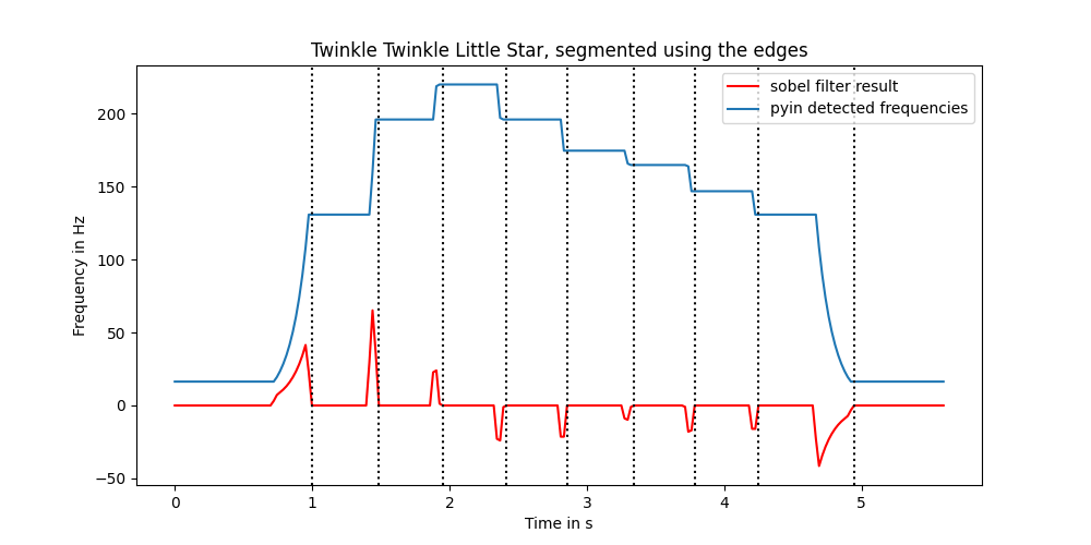
And if I have an edge detector, I can slice the notes time wise. If I can slice the notes, I can average them, median them, stick them in a stew, whatever I need to estimate them best.
The Sobel filter is actually pretty nice. Not only is it better at detecting the edges here, it seems to have as a side property that the peak rises if the next note rises and vice-versa, drops if the next note is lower. Which could be useful down the line.
I am a bit worried of what it will do to a "real" signal though.
But let's finish what we came here for. Let's separate the groups. We just have to find the 0 values after any value different to 0 here (one more thing that might change later on, but let's start simple.).
sobelified_f0=sim.sobel(f0)

a = 0
note_shifts=[]
for i,v in enumerate(sobelified_f0):
    if v!=0:
        a=v
    if a!=0 and v==0:
        note_shifts.append(times[i])
        a=0

f,a = plt.subplots()
a.plot(times,sim.sobel(f0),label="sobel filter result",color="r")
a.plot(times,f0,label="pyin detected frequencies")
a.legend()
a.set_xlabel("Time in s")
a.set_ylabel("Frequency in Hz")
a.set_title("Twinkle Twinkle Little Star, segmented using the edges")

for v in note_shifts:
    a.axvline(v,color="k",linestyle=":")

f.set_size_inches(10,5)
f.savefig("twinkle_twinkle_little_star_segmented.png")

Then for now, let's just use the median on the data in between:
music_sheet = []
for i in range(len(note_shifts)-1):
    median_frequency = np.median(f0[(note_shifts[i]<=times) & (times<=note_shifts[i+1])])
    music_sheet.append(librosa.hz_to_note(median_frequency))

" ".join(music_sheet)
And here we go! It yields the expected 'C3 G3 A3 G3 F3 E3 D3 C3'.
Next time, let's condense the program and see how it performs on a voice sample.
previously
Boxcar functions
audioFlux pitch estimation example
Twinkle, Twinkle, Little Star
order filter
some slides I found online on filtering
⋅∽⋅∼⋅∽⋅∼⋅∽⋅∼⋅∽⋅∼⋅∽⋅∼⋅∽⋅∼⋅∽⋅∼⋅∽⋅∼⋅∽⋅∼⋅∽⋅∼⋅∽⋅∼⋅∽⋅∼⋅∽⋅∼⋅∽⋅∼⋅∽⋅∽⋅∼⋅∽⋅∽⋅